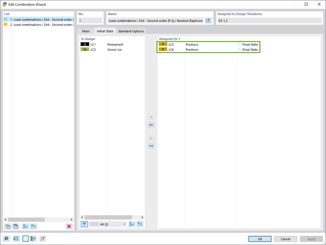
The combination wizard provides you with the option to consider more than one initial state. RFEM and RSTAB allow you to specify different initial states (prestress, form-finding, strain, and so on) for the target combinations in the combinatorics.
You can thus, for example, generate load states on the basis of a form-finding analysis with varying imperfections.
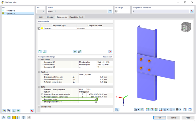
In the Steel Joints add-on, you have this option to consider the preloaded bolts in the calculation of all components.
You can easily activate the prestress using the check box in the bolt parameters, and it has an impact on the stress-strain analysis as well as the stiffness analysis.
Go to Explanatory Video
Once you activate the Form-Finding add-on in the Base Data, a form-finding effect is assigned to the load cases with the load case category "Prestress" in conjunction with the form-finding loads from the member, surface, and solid load catalog. This is a prestress load case. It thus mutates into a form-finding analysis for the entire model with all member, surface, and solid elements defined in it. You reach the form-finding of the relevant member and membrane elements amid the overall model by using special form-finding loads and regular load definitions. These form-finding loads describe the expected state of deformation or force after the form-finding in the elements. The regular loads describe the external loading of the entire system.

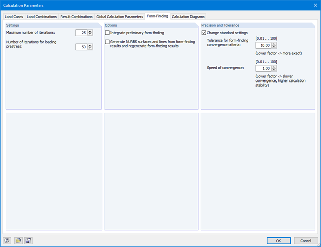
Do you know exactly how the form-finding is performed? First, the form-finding process of the load cases with the load case category "Prestress" shifts the initial mesh geometry to an optimally balanced position by means of iterative calculation loops. For this task, the program uses the Updated Reference Strategy (URS) method by Prof. Bletzinger and Prof. Ramm. This technology is characterized by equilibrium shapes that, after the calculation, comply almost exactly with the initially specified form-finding boundary conditions (sag, force, and prestress).
In addition to the pure description of the expected forces or sags on the elements to be formed, the integral approach of the URS also enables a consideration of regular forces. In the overall process, this allows, for example, for a description of the self-weight or a pneumatic pressure by means of corresponding element loads.
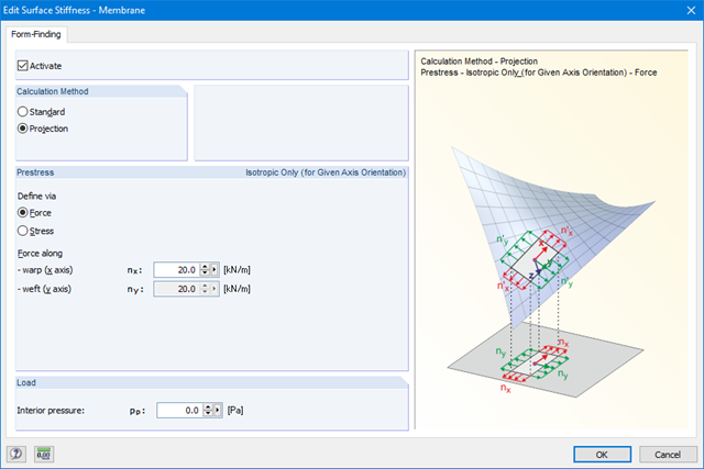
All these options give the calculation kernel the potential to calculate anticlastic and synclastic forms that are in an equilibrium of forces for planar or rotationally symmetric geometries. In order to be able to realistically implement both types individually or together in one environment, the calculation provide you with two ways to describe the form-finding force vectors:
- Tension method - description of the form-finding force vectors in space for planar geometries
- Projection method - description of the form-finding force vectors on a projection plane with fixation of the horizontal position for conical geometries

The form-finding process gives you a structural model with active forces in the "prestress load case" This load case shows the displacement from the initial input position to the form-found geometry in the deformation results. In the force or stress-based results (member and surface internal forces, solid stresses, gas pressures, and so on), it clarifies the state for maintaining the found form. For the analysis of the shape geometry, the program offers you a two-dimensional contour line plot with the output of the absolute height and an inclination plot for the visualization of the slope situation.
Now, a further calculation and structural analysis of the entire model is performed. For this purpose, the program transfers the form-found geometry including the element-wise strains into a universally applicable initial state. You can now use it in the load cases and load combinations.

- Automatic consideration of masses from self-weight
- Direct import of masses from load cases or load combinations
- Optional definition of additional masses (nodal, linear, or surface masses, as well as inertia masses) directly in the load cases
- Optional neglect of masses (for example, mass of foundations)
- Combination of masses in different load cases and load combinations
- Preset combination coefficients for various standards (EC 8, SIA 261, ASCE 7,...)
- Optional import of initial states (for example, to consider prestress and imperfection)
- Structure Modification
- Consideration of failed supports or members/surfaces/solids
- Definition of several modal analyses (for example, to analyze different masses or stiffness modifications)
- Selection of mass matrix type (diagonal matrix, consistent matrix, unit matrix), including user-defined specification of translational and rotational degrees of freedom
- Methods for determining the number of mode shapes (user-defined, automatic - to reach effective modal mass factors, automatic - to reach the maximum natural frequency - only available in RSTAB)
- Determination of mode shapes and masses in nodes or FE mesh points
- Results of eigenvalue, angular frequency, natural frequency, and period
- Output of modal masses, effective modal masses, modal mass factors, and participation factors
- Masses in mesh points displayed in tables and graphics
- Visualization and animation of mode shapes
- Various scaling options for mode shapes
- Documentation of numerical and graphical results in printout report

- Calculation of models consisting of member, shell, and solid elements
- Nonlinear stability analysis
- Optional consideration of axial forces from initial prestress
- Four equation solvers for an efficient calculation of various structural models
- Optional consideration of stiffness modifications in RFEM/RSTAB
- Determination of a stability mode greater than the user-defined load increment factor (Shift method)
- Optional determination of the mode shapes of unstable models (to identify the cause of instability)
- Visualization of the stability mode
- Basis for determining imperfection
.png?mw=640&hash=688fdfc8af4828c08e9851cddb103a1e86cb899a)
- Form-finding of:
- tension-loaded membrane and cable structures
- compression-loaded shell and beam structures
- mixed tension- and compression-loaded structures
- Consideration of gas chambers between surfaces
- Interaction with supporting structure (substructure design according to various standards)
- Surfaces as a 2D and members as a 1D element
- Definition of different prestress conditions for surfaces (membranes and shells)
- Definition of forces or geometrical requirements for members (cables and beams)
- Consideration of individual loads (self‑weight, inner pressure, and so on) in the form‑finding process
- Temporary support definitions for the form-finding process
- Automatic preliminary form-finding of membrane surfaces (more information...)
- Definition of isotropic or orthotropic material for structural analysis
- Optional definition of free polygon loads
- Transformation of form‑found shape elements into NURBS surface elements
- Possibility of combined form-finding by integration of preliminary form-finding
- Graphical evaluation of the new form using colored coordinates and inclination plots
- Complete documentation of the calculation including user-defined adaptive evaluation figures
- Optional export of the FE mesh as a DXF or Excel file
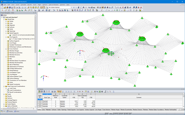
The results of the form‑finding process are a new shape and corresponding inner forces. The usual results, such as deformations, forces, stresses, and others can be displayed in the RF‑FORM‑FINDING case.
This prestressed shape is available as the initial state for all other load cases and combinations in the structural analysis.
For more ease when defining load cases, the NURBS transformation can be used (Calculation Parameters/Form-Finding). This feature moves the original surfaces and cables into position after form‑finding.
By using the grid points of surfaces or the definition nodes of NURBS surfaces, free loads can be situated on selected parts of the structure.
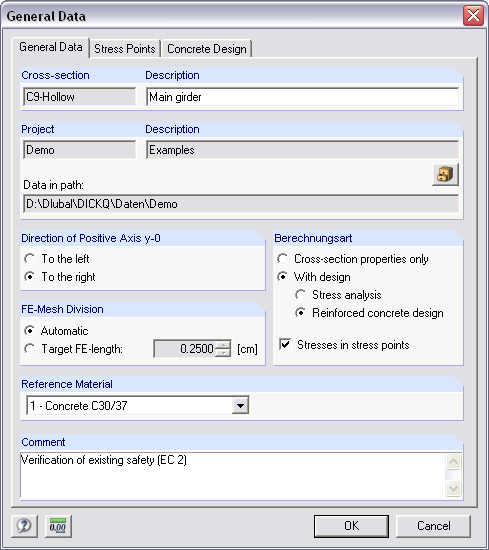
The form-finding function can be activated in the General Data dialog box, Options tab. Prestresses (or geometrical requirements for members) can be defined in the parameters for surfaces and members. The form‑finding process is performed by calculation of an RF‑FORM‑FINDING case.
Steps of the working sequence:
- Creation of a model in RFEM (surfaces, beams, cables, supports, material definition, and so on)
- Setting of required prestress for membranes and force or length/sag for members (for example, cable)
- Optional consideration of other loads for the form-finding process in special form‑finding load cases (self‑weight, pressure, steel node weight, and so on)
- Setting of loads and load combinations for further structural analyses
After starting the calculation, the program performs form‑finding on the entire structure. The calculation takes into account the interaction between the form‑finding elements (membranes, cables, and so on) and the supporting structure.
The form-finding process is performed iteratively as a special nonlinear analysis, inspired by URS (Updated Reference Strategy) by Prof. Bletzinger / Prof. Ramm. This way, shapes in equilibrium are obtained considering the pre‑defined prestress.
Furthermore, this method allows you to consider individual loads such as self‑weight or internal pressure for pneumatic structures in the form‑finding process. The prestress for surfaces (for example, membranes) can be defined using two different methods:
- Standard method - prescription of required prestress in a surface
- Projection method - prescription of required prestress in the projection of a surface, stabilization especially for conical shapes
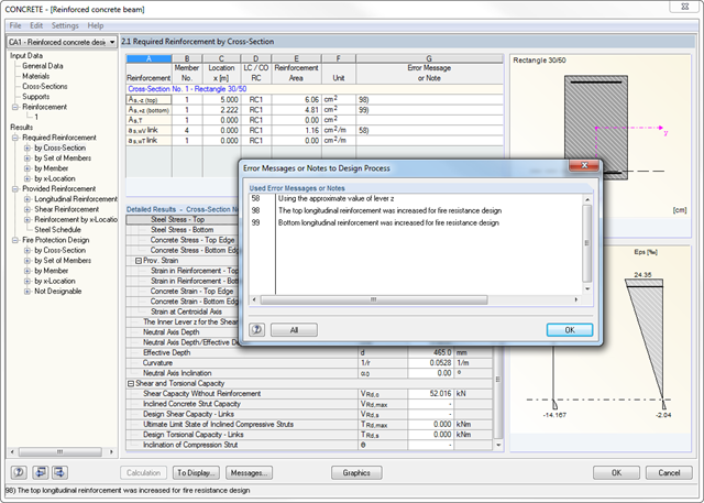
Before the calculation starts, you should check the input data using the program function. Then, the CONCRETE add‑on module searches the results of relevant load cases, load as well as result combinations. If these cannot be found, RSTAB starts the calculation to determine the required internal forces.
Considering the selected design standard, the required reinforcement areas of the longitudinal and the shear reinforcement as well as the corresponding intermediate results are calculated. If the longitudinal reinforcement determined by the ultimate limit state design is not sufficient for the design of the maximum crack width, it is possible to increase the reinforcement automatically until the defined limit value is reached.
The design of potentially unstable structural components is possible using a nonlinear calculation. According to a respective standard, different approaches are available.
The fire resistance design is performed according to a simplified calculation method in compliance with EN 1992‑1‑2, 4.2. The module uses the zone method mentioned in Annex B2. Furthermore, you can consider the thermal strains in the longitudinal direction and the thermal precamber additionally arising from asymmetrical effects of fire.
- Design according to EN 13480-3, ASME B31.1-2012, and ASME B31.3-2012
- Check of the minimum required wall thickness of the pipes, taking into account manufacturing allowances, corrosion, and welding factor
- Analysis of stresses due to sustained loads, sustained and occasional loads as well as due to thermal expansion
- Result documentation with tables and graphics in the RFEM printout report
- Automatic consideration of masses from self-weight
- Direct import of masses from load cases or load combinations
- Optional definition of additional masses (nodal, linear, surface masses, as well as inertia masses)
- Combination of masses in different mass cases and mass combinations
- Preset combination coefficients according to EC 8
- Optional import of normal force distributions (in order to consider prestress, for example)
- Stiffness modification (for example, deactivated members or stiffnesses can be imported from RF-/CONCRETE)
- Consideration of failed supports or members
- Definition of several natural vibration cases (for example, to analyze different masses or stiffness modifications)
- Results of eigenvalue, angular frequency, natural frequency, and period
- Determination of mode shapes and masses in nodes or FE mesh points
- Results of modal masses, effective modal masses, and modal mass factors
- Visualization and animation of mode shapes
- Various scaling options for mode shapes
- Documentation of numerical and graphical results in the printout report
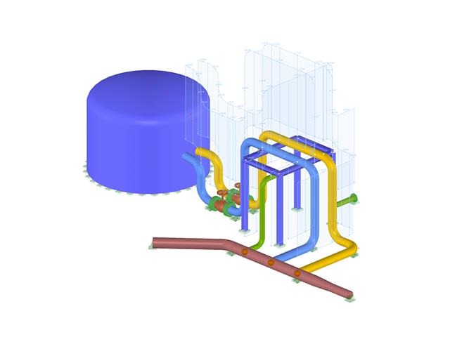
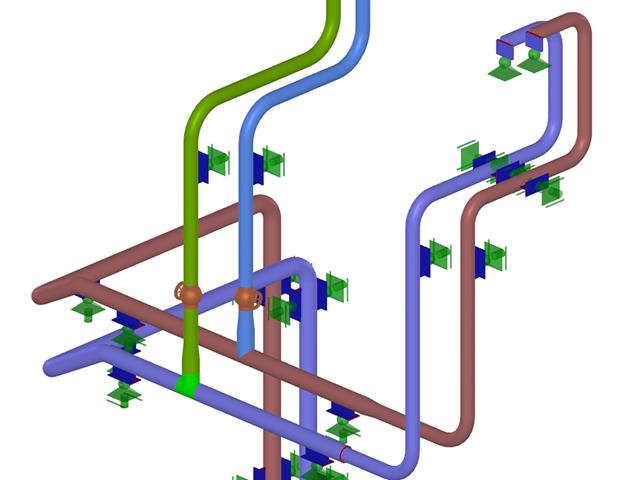
- Graphical input of piping systems and piping components
- Illustrative visualization of piping systems and piping components in RFEM graphic window
- Comprehensive libraries for piping cross‑sections and materials
- Comprehensive libraries for flanges, reducers, tees, and expansion joints
- Consideration of piping structure (insulation, lining, tin‑plate)
- Automatic calculation of stress intensification factors and flexibility factors
- Specific piping action categories for load cases
- Optional automatic combinatorics of load cases
- Consideration of material properties (modulus of elasticity, coefficient of thermal expansion) either during operating temperature (default setting) or during reference (assembly) temperature of material
- Consideration of strain and uplift due to pressure (Bourdon effect)
- Interaction between the supporting structure and the piping system
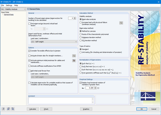
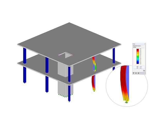
First of all, it is necessary to select a load case or combination whose axial forces are to be used in the stability analysis. It is possible to define another load case to, for example, For example, you have to consider an initial prestress.
Then, you can select the linear or non-linear analysis to be performed. Depending on the application, you can use a direct calculation method, such as according to Lanczos or the ICG iteration method. Members not integrated in surfaces are usually displayed as member elements with two FE nodes. It is not possible to determine the local buckling of single members on these elements. Therefore, you have the option to divide members automatically.

If there is a load case or load combination in the program, the stability calculation is activated. You can define another load case in order to consider initial prestress, for example.
For this, you need to specify whether to perform a linear or nonlinear analysis. Depending on the case of application, you can select a direct calculation method, such as the Lanczos method or the ICG iteration method. Members not integrated in surfaces are usually displayed as member elements with two FE nodes. With such elements, the program cannot determine the local buckling of single members. That's why you have the option to divide members automatically.
The global calculation assigns the stiffness determined by means of the selected composition and the glass geometry to each surface. Then, the calculation proceeds using the plate theory. It is possible to select whether the shear coupling of layers should be considered.
In the case of the local calculation, you can further specify 2D or 3D calculation. Two-dimensional calculation means that the single-layer or laminated glass is modeled as a surface, whose thickness is calculated on the basis of the selected structure and glass geometry (using the plate theory). Similarly to the global calculation, you can optionally consider shear coupling of layers.
The 3D calculation uses solids in the model to substitute each composition layer. This way, the results are more accurate, but the calculation may take more time.
It is possible to model insulating glass only if local calculation is selected. The gas layer is always modeled as a solid element, so it is necessary to design individual insulating glass parts independently of the surrounding structure. The ideal gas law (thermal equation of state of ideal gases) is considered for the calculation and the third-order analysis.
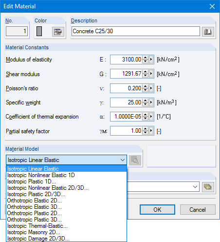
Structures are entered as 1D, 2D, or 3D models. Member types such as beams, trusses, or tension members facilitate the definition of member properties. For modeling surfaces, RFEM provides For example, the types Standard, Orthotropic, Glass, Laminate, Rigid, Membrane, and so on, are available.
Furthermore, RFEM can select among the material models Isotropic Linear Elastic, Isotropic Plastic 1D/2D/3D, Isotropic Nonlinear Elastic 1D/2D/3D, Orthotropic Elastic 2D/3D, Orthotropic Plastic 2D/3D (Tsai-Wu 2D/3D), and Isotropic Thermal -elastic, Isotropic Masonry 2D, and Isotropic Damage 2D/3D.
It is possible to freely model a cross-section using surfaces limited by polygonal lines, including openings and point areas (reinforcements). Alternatively, you can use the DXF interface to import the geometry. An extensive material library facilitates the modeling of composite cross-sections.
Definition of limit diameters and priorities allows for a curtailment of reinforcements. In addition, you can consider the respective concrete covers and prestresses.
- Calculation of models consisting of member, shell, and solid elements
- Import of axial forces from a load case or combination
- Non-linear stability analysis
- Optional consideration of axial forces from initial prestress
- Four equation solvers for effective calculation of various structural models
- Optional consideration of stiffness modifications in RFEM
- Calculation of buckling modes of unstable models
- Determination of stability mode greater than the user-defined load increment factor (Shift method)
- Optional determination of the mode shapes of unstable models (to identify the cause of instability)
- Visualization of stability mode
- Basis for analysis using imperfect equivalent structures in RF-IMP